Home / Posts / Backcountry travel time part1

Backcountry Travel Time Estimation – Part 1

Backcountry travel time estimation is the discipline of looking at a hike, ski tour, or other outdoor objective, and figuring out how long it will take. It’s an art, not really a science, and I’m going to use that fact to justify my “artistic” use of statistical techniques to evaluate two specific methods for doing this estimation, the Munter method and Tobler’s Hiking function.

In typical fashion, I generate far more questions than conclusions, and may post some further analysis in a follow up post.

If you’re interested, check out the code for this analysis.

Background: Travel time estimation in Caltopo

I first came across the idea of backcountry travel time estimation as a feature of the popular mapping software CalTopoThis feature allows you to generate a detailed travel plan with travel time estimates for a planned route.

Here’s how the travel plan feature works:

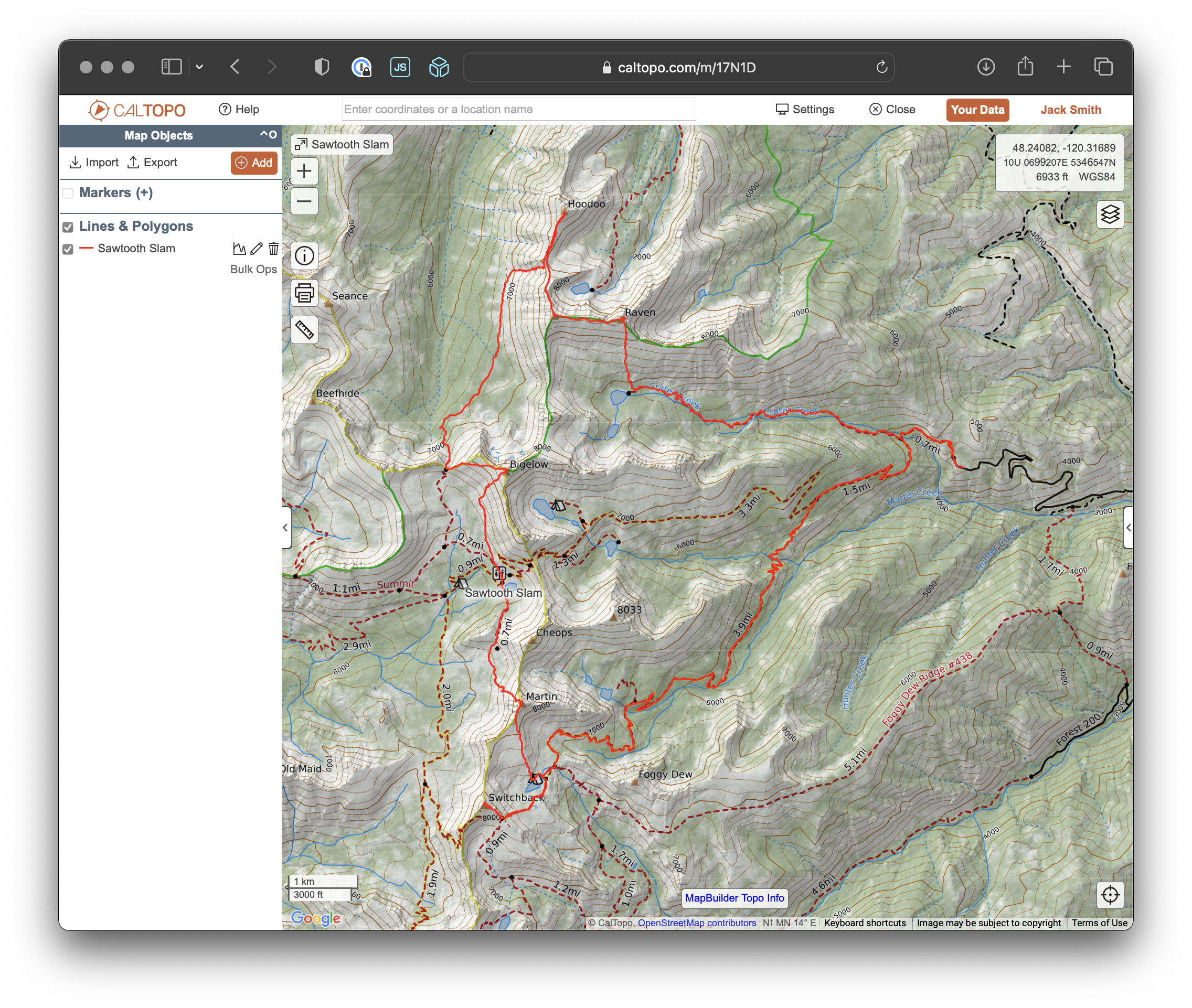
First, we put in a track that we’re planning on following. For example, here is a track for the “Sawtooth Slam” which is a popular linkup in the Lake Chelan sawtooth wilderness here in Washington.

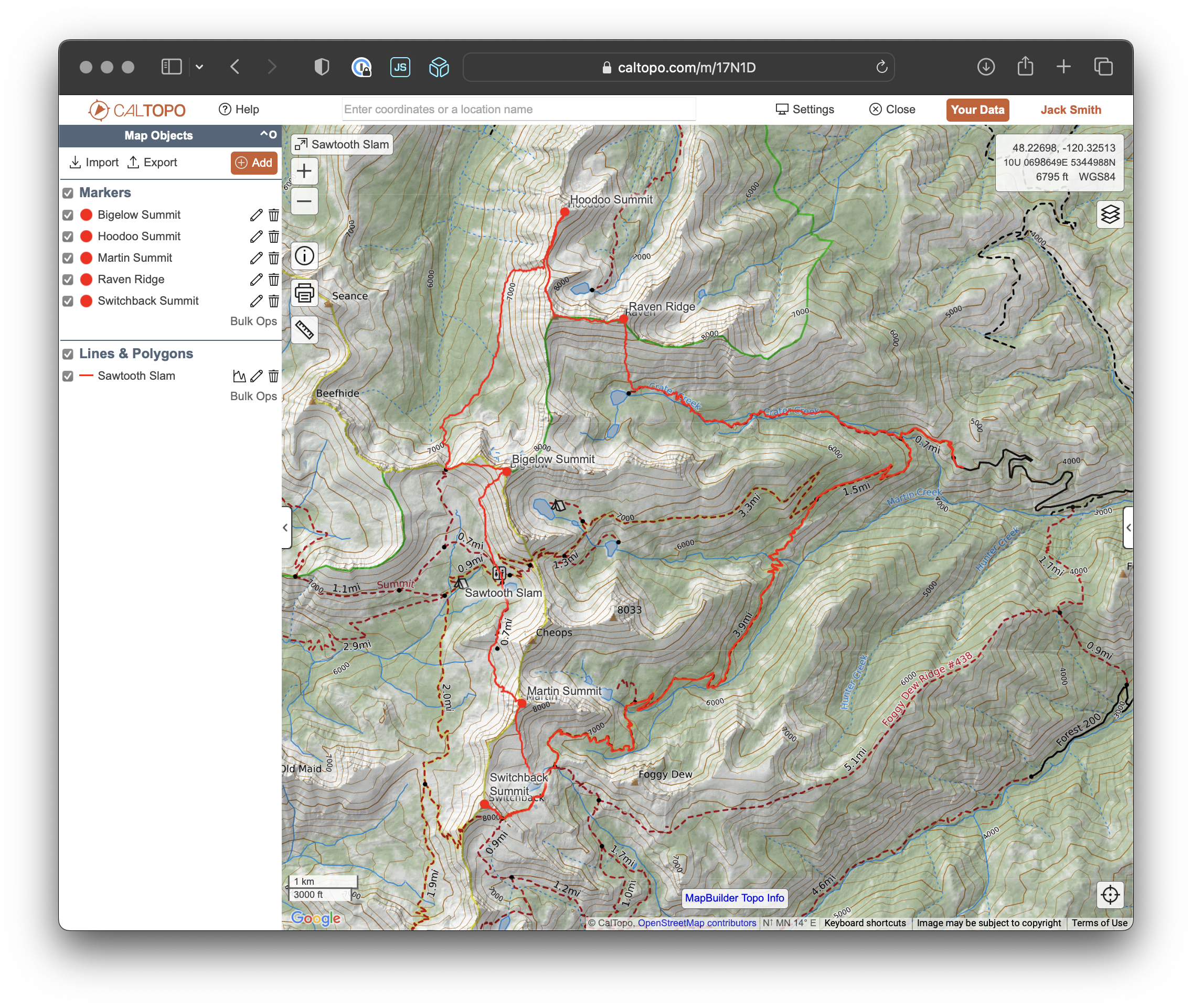
Next, we add any relevant waypoints along the route that we care about. Here, I’ve added markers for all the summits included in the linkup:

Finally, we ask CalTopo to generate a travel plan for our track. It spits out stats for each leg of our trip and projects a travel time. Here, we see that this hike is projected to take about 20 hours.

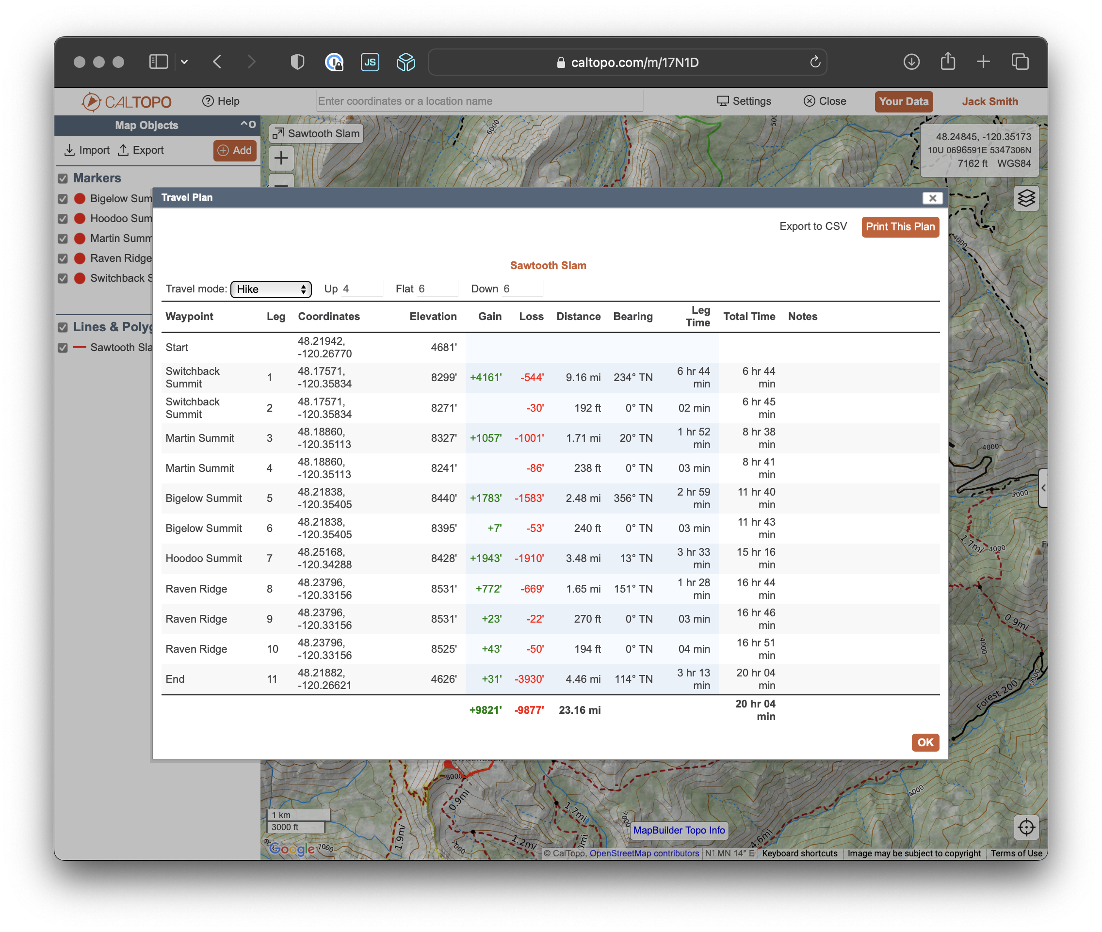
If we lookup the Fastest Known Time for this route. We see it’s an impressive showing of 9hrs and 22min by Nathan Longhurst! For Nathan at least, this travel time estimation is off by quite a bit!

This feature intrigued me because of its obvious utility as a planning tool. So I wanted to learn how it worked and what it’s limitations are. The caltopo documentation for this feature explains that the calculations it produces are created by a technique called the Munter Method.

What are the methods for travel time estimation?

The Munter Method: A back of the napkin approach from a mountaineering legend

Legendary mountain guide Werner Munter is best known for his popularization of a belay hitch now refered to as a Munter Hitch by climbers. As a guide, he developed a method for estimating how long legs of a trip would take, and this method now also bears his name. Munter’s method is optimized for simplicity and easy calculation in the field. This is the method adopted by CalTopo in their travel plan feature.

Munter’s equation:

\[\text{TIME (hours)} = \frac{\lvert \text{DISTANCE(km)} + \frac{\text{ELEVATION CHANGE(m)}}{100} \rvert}{\text{RATE}}\]

The art of the Munter method is that the RATE parameter needs to be adjusted for our personal rate of travel. For flat ground where there is no elevation change, the elevation change term drops out which means RATE just is our speed in km/hr. The adjustment for elevation change reflects the fact that as the trail gets steeper, it becomes harder to maintain the same pace, either because of the increased effort required for uphill travel or the need for caution during downhill travel. This should make intuitive sense to anyone who’s been on a steep trail before.

For the purpose of visualization, I’m going to switch from talking about travel time and elevation change to talking about pace as a function of slope grade. This makes visualizing a pace function such as Munter’s equation easier. I’ll also switch units from hours and km to meters per second, since it should be very intuitive what a given pace feels like in those units.

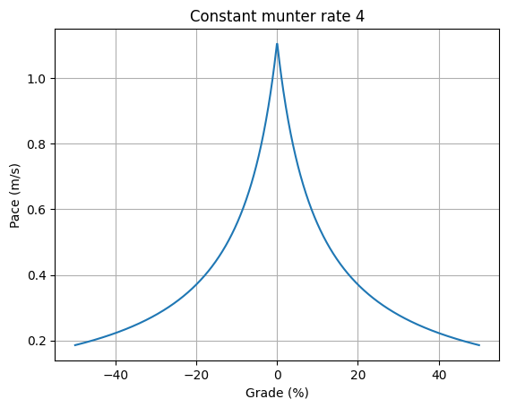
As an example: Here is the pace function that we get for the Munter equation with RATE=4. It shows the basic shape we would expect, on flat ground we go fast (around 1 m/s) and as the trail gets steeper, we slow down significantly.

The Munter method was designed to be flexible for use by both hikers and skiers, and this single rate function clearly won’t work well for skiing because when we move downhill on skis, we can go very fast on moderate downhill slopes.

To account for this and allow more fine customization, the Munter method specifies that you should break your trip into segments, classify each as uphill, flat, or downhill, and apply a different rate to each segment.

The standard rate schedule used by CalTopo and others are:

Activity	Down	Flat	Up
Hike	6	6	4
Ski	10	6	4
Bushwack	2	2	2

In this post, I’ll describe the parameters in an ordered tuple so hike will be Munter (6,6,4).

How do we classify a segment as uphill, downhill, or flat? For Werner Munter this was simple, you just looked at the topographic map and made your best judgement for where segments start and end to best fit into these categories.

CalTopo made the decision to analyze tracks by breaking them into 50m chunks, and categorizing them into the downhill, flat, and uphill bins if their grade was less than -5%, between -5% and 5%, and greater than 5%. I will make the exact same choice for the rest of this post.

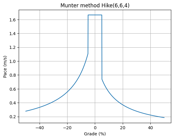
Here is the full, piecewise Munter pace function using the standard rate parameters for hiking:

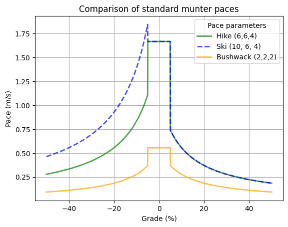
Here is a comparison of all the standard Munter pace schedules. Notice how downhill skiing gets a significant rate boost vs hiking downhill. Also notice, for bushwhacking, it doesn’t matter if we’re moving up or downhill, our problem is going to be vegetation anyways.

Tobler’s Hiking Function: An idea from the GIS wizard

Tobler’s hiking function is another approach to the same problem, created by professor of geography Waldo R. Tobler. Tobler is apparently a legendary figure in geography, and an early pioneer in GIS. He seems to be best known for “The first law of geography” which states:

Everything is related to everything else, but near things are more related than distant things

Maybe this is a profound statement among geographers? I’m not so sure how I would feel about this being the best known thing I ever said, especially if I had a body of work like Tobler’s. I’m not here to judge though, except for methods of travel time estimation, that is.

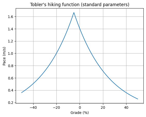
Tobler gathered data from his friend who was a hiker, and from the data produced Tobler’s Hiking Function:

\[VELOCITY(km/hr)=6e^{-3.5\left|GRADE+0.05\right|}\]

Let’s take a look at what the parameters to this function mean. For the unfitted function with free parameters:

\[VELOCITY(km/hr)=P e^{-D\left|GRADE+B\right|}\]

P is our maximum speed in km/hr
D is our decay parameter, it controls how quickly our speed is reduced as we get further from the optimal pace. A larger value here means our pace takes a bigger hit in steeper terrain.
B is the bias parameter, it shifts our function left or right and controls at which grade we realize our maximum speed. A small positive value here means that our maximum pace is on a slightly negative slope, which intuitively makes sense.

When we plot Tobler’s function the same way we plotted Munter’s, we see a similar shape, but with the characteristic bias:

Comparing Tobler’s Function and the Munter Method

Let’s overlay Tobler’s function and the Munter hike function on the same graph so we can see the different predictions they make.

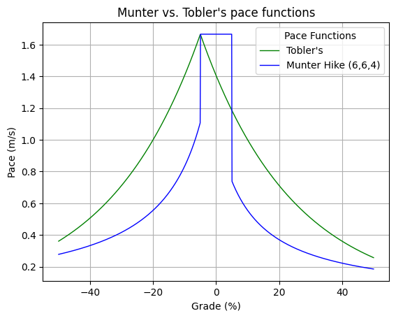
We notice some striking differences!

Tobler’s function predicts significanly slower paces when traveling on flat or slightly uphill segments.
Tobler’s function is significantly more optimistic about our pace at higher grades of travel both uphill and downhill!

Comparing both methods on Mt. Si

Let’s work through both methods on the popular Seattle area hike Mount Si. Here is the elevation profile I get from CalTopo:

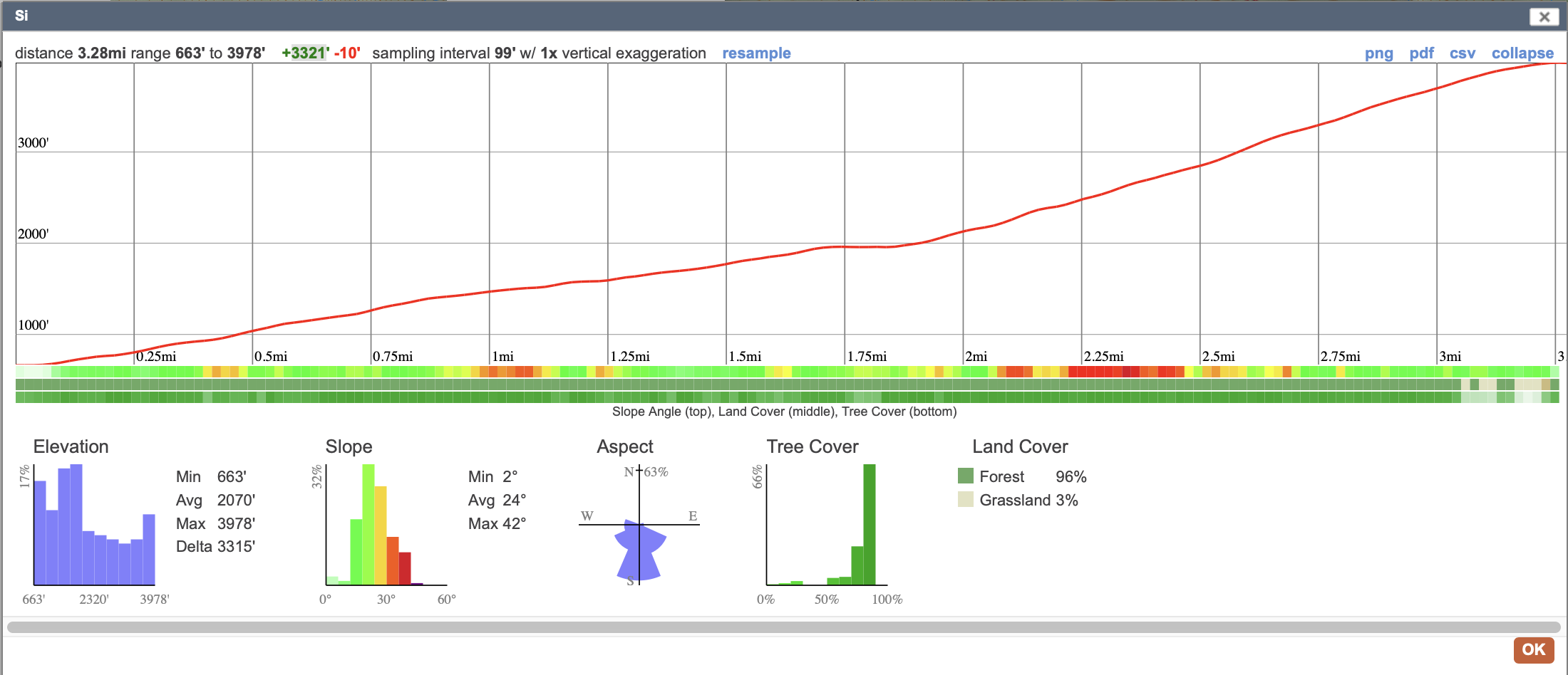
The trail is 3.28 miles long, and has 3321 feet of elevation gain. In meters, thats 5,279 horizontal, and 1,012 vertical. The trail has a relatively consistent grade of around 20%, and only has one small flat part, which we will ignore.

Calculations for Munter Method:

\[\begin{aligned} \text{Uphill time:} \quad \frac{5.279 + \frac{1012}{100}}{4} &= 3.84\text{ hrs} \\ \text{Downhill Time:} \quad \frac{5.279 + \frac{1012}{100}}{6} &= 2.56\text{ hrs} \\ \text{Total Time:} \quad 3.84\text{ hrs} + 2.56\text{ hrs} &= 6.41\text{ hrs} \end{aligned}\]

Calculations for Tobler’s Function:

\[\begin{aligned} \text{Velocity uphill:} \quad 6 * e^{-3.5 * abs(0.1917 + 0.05)} &= 2.574\text{ km/hr} \\ \text{Uphill time:} \quad \frac{1}{2.574\text{ hr/km}} * 5.28\text{ km} &= 2.05\text{ hrs} \\ \text{Velocity downhill:} \quad 6 * e^{-3.5 * abs(-0.1917 + 0.05)} &= 3.65\text{ km/hr} \\ \text{Downhill time:} \quad \frac{1}{3.65\text{ hr/km}} * 5.28\text{ km} &= 1.45\text{ hrs} \\ \text{Total Time:} \quad 2.05\text{ hrs} + 1.45\text{ hrs} &= 3.50\text{ hrs} \end{aligned}\]

These are radically different! For me at least, Tobler’s method is much closer to how long this hike would take me at a normal hiking pace. This maybe should not be that suprising, since Munter developed his heuristic for guiding mountaineering trips, which are generally far more strenuous and often off trail in high alpine areas, Tobler developed his for hiking on trails.

This comparison is a clear win for Tobler’s function. To learn more about how these methods actually stack up in practice, we need some empirical data.

Empirical Data

Gathering my Strava Data

I upload all my outdoor activities to Strava and (thanks to GDPR) I can download all the raw gps data I’ve collected. In the rest of this post, this will be the dataset I use to evaluate the standard pace functions. For now, I will only use my own data for analysis. However, if you have similar data and would like to perform some analysis, please contact me or take a look at my code to try it yourself.

When I export my Strava data, I get a folder that looks like this:

.
├── activities
│   ├── 1742358089.gpx
│   ├── 1751453728.gpx
│   ├── 1759584243.gpx
│   ├── 1824415774.gpx
│   ├── 1841831332.gpx
│   ├── 1846849354.gpx
│   ├── 1847032434.fit.gz
│   ├── 1847034807.fit.gz
│   ├── ... 
├── activities.csv
├── applications.csv
├── bikes.csv
├── blocks.csv
├── ...

There’s actually a ton more data in here, including all my uploaded photos, I’m just showing the stuff that’s relavent to us. In particular, the activities directory contains all the raw GPS data collected by whatever device I was using to record and the activities.csv file contains the metadata. This metadata was useful because it contains the particular type of sport I was doing, so it let me filter the tracks to the two we care about: Hiking and Backcountry Skiing.

Note: My hiking tracks probably include some bushwhacking, but in the interest of time, I did not manually break each track into chunks based on terrain type. This could be an interesting followup though, and may be useful for developing new rules of thumb.

Getting this data into usable shape was a pain, and I’m not going into all the detail here to save time. Some of these activities were missing elevation data making them useless. Many of them were recorded with a gps device that creates .fit files, and those needed to be converted to .gpx files.

In the end, I ended up with 33 hiking tracks and 38 backcountry ski tracks. I may update this analysis at some point in the future to include more recent activities.

A First Look at my data

The first thing I did with the data is broke each track into 50m chunks (using the same methodology as caltopo) and plotted each chunk in the grade vs pace space. Here’s what we get:

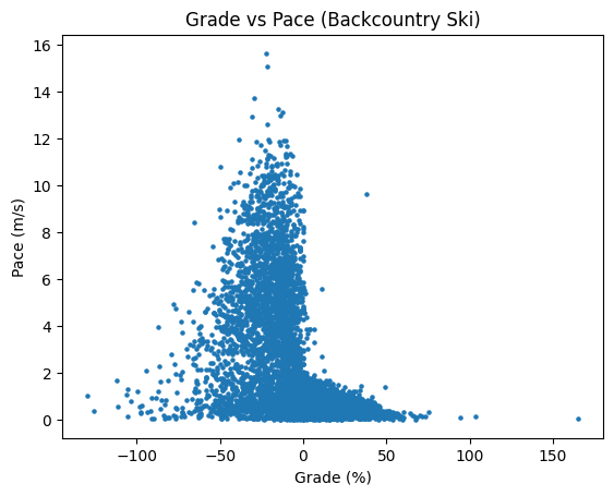
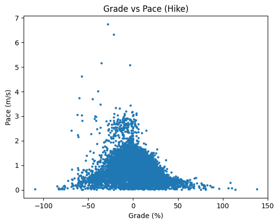
A few interesting observations immediately:

Skiing downhill is radically faster than skinning up even a very slight grade. Completely unsurprising, but a good sanity check of the data.
Hiking has far less discontinuity between uphill and downhill, but still some. This is probably because if I do jog during a hike, it’s very likely to be on a downhill section.
Our maximum hiking rates are indeed at a grade slightly less than 0%, this is another good sign for Tobler’s function.

Ultimately, the scatterplot is pretty messy. There’s too much data to really see where our speed is distributed inside that big mass of blue dots. Instead, let’s break the grades up into 30 bins, then we can plot the median and quartiles for our pace data:

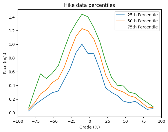
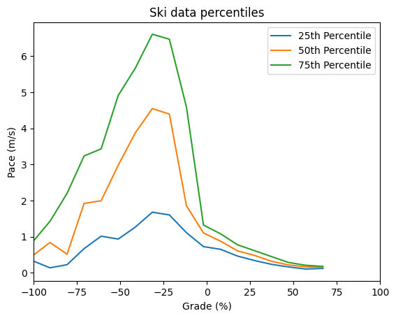
A few more observations based on the data:

Skiing has a maximum pace at much steeper grades than hiking. Again, unsurprising.
Skiing is really fast! I should keep doing that to get down the mountain when I can. Even less surprising.
Our ski pace slows down as we move from -25% grades to 0% grades. This is probably because as we get flatter, friction slows us down more. Annoying, I’m reliving those segments now.
Skiing uphill looks pretty similar to hiking, paces are closely distributed.
Ski pace has a much wider distribution downhill than hiking downhill. This is probably due to the wide variation in ski conditions. Skiing an open slope of perfect light snow will drag that green line way up. A horrible sheet of ice with cliffs below will drag the blue line way down. We probably shouldn’t expect any formula to work all that well for downhill ski sections.

A visual comparison of My Data and the Standard Functions

For fun, let’s superimpose the percentiles plots from my data with the standard pace functions and see if we can spot anything interesting.

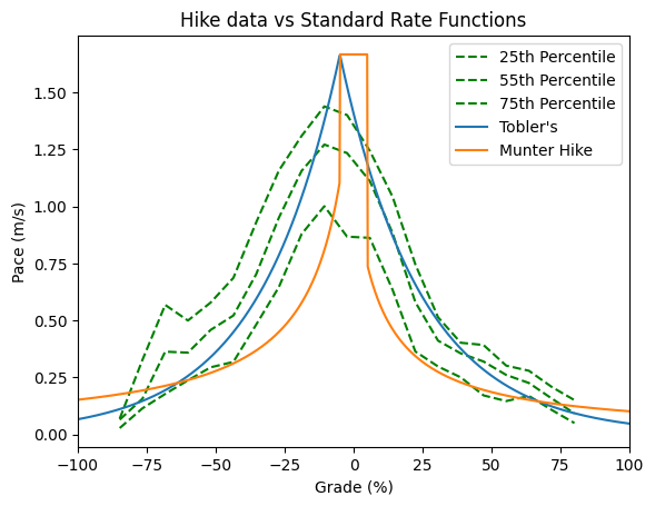
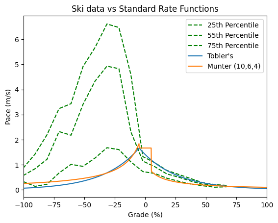
Here’s what I see:

Tobler’s function fits my hiking data really well right out of the box, though it’s a little optimistic about my max speed. This may be due to the fact that I take breaks to eat lunch, filter water, and take photos on many of my hikes (we’ll work on that problem in detail later).
Both pace functions dramatically underestimate the speed of downhill skiing. This was initially surprising to me. How can these work even a little if they get these downhill speeds so wrong? The answer turns out to be simple: Downhill speed isn’t that important for predicting overall time, because it’s over so fast! If we spend 80% of our trip toiling uphill, being off by even a large margin on the downhill section matters far less than accuracy on the uphill.

Quantitative comparison of the standard functions

Just looking at the data is interesting, but what we really care about is predictive power. To evaluate this, I predicted the time that each of my tracks would take using both Munter’s Method and Tobler’s Function.

I then evaluated the error, normalizing by the actual track time as follows:

\[\text{Error} = \frac{\text{Predicted Time} - \text{Actual Time}}{\text{Actual Time}}\]

Thus, if a method yields an error of 0.25 for a given track, the predicted time was 25% longer than the actual time.

Here are what these errors look like for our Hike Tracks:

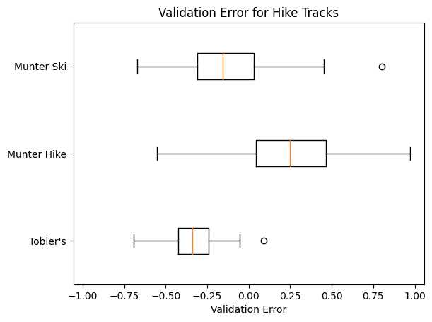
Observations:

Tober’s is certainly a bit optimistic, remember what we learned earlier, our pace in the slowest parts matters the most. Tobler’s was a good visual fit to our data, which means it’s probably very good at answering the question “Given this 50m chunk, predict the speed” but for the actual problem, we want those slow chunks to get more weight.
Despite this, our results with the munter method are all over the place. Look at that spread of errors! Tobler’s might be a little too optimistic, but the clustering of errors is far better. Here’s the first real conclusion I can offer, if you’re going on a hike and want to use a standard function: Tobler’s is a better bet.

How about our ski data? Here’s what the errors look like there:

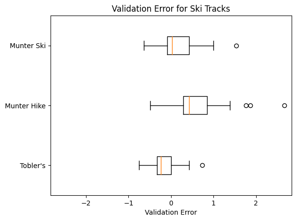
Observations:

Ouch! Look at that scale! Predicting ski travel times is way more difficult to do with any accuracy. Keep this in mind if you want to apply these methods in your own planning.
Despite the huge error bars, the standard Munter ski function, and the standard Tobler’s function do sort of okay? At least they’re close-ish to calibrated?
As far as recommendations go, I don’t think the data is conclusive at all about which standard method works best.

Predicting Moving Time Instead of Total Time

I’ve alluded to this through the last section, but our analysis up to this point has neglected a major source of variation in our activity times: Taking breaks!

Sometimes, I take a break because I’m exhausted and need to rest in order to continue, but that’s not the most common reason. More often, I take breaks because I want to eat lunch, take a photo, or enjoy a view. The important realization is that the number and duration of breaks has less to do with terrain than it does with conditions, social dynamics, and the goals for a hike or tour.

One consequence of this realization, is that we may have better luck predicting the “moving time” for our track rather than the “total time”. Let’s put that theory to the test by removing breaks from our tracks and running our analysis again.

Note: Removing breaks is also going to slice out breaks that actually are essential for the trip, things like roping up before getting on a glacier. If we use this methodology, we had better have a good idea about how many breaks we need to take and how long they will be!

Break Removal or How To Get Faster Using Code

Let’s use one particular track from my data, which is a hike that connects Star Peak, Courtney Peak, and Oval Peak in the Lake Chelan Sawtooth Wilderness. According to the Fastest Known Time (FKT) website at time of writing, Fabien Le Gallo has the FKT for this route at 10 hours, 20 minutes, and 58 seconds.

I stack up quite a bit slower than Fabien at 14 hours, 47 minutes, and 24 seconds. Unlike Fabien (who I assume must have taken no breaks whatsoever) I took some breaks along the way. This is really clear from a plot of my elevation over time:

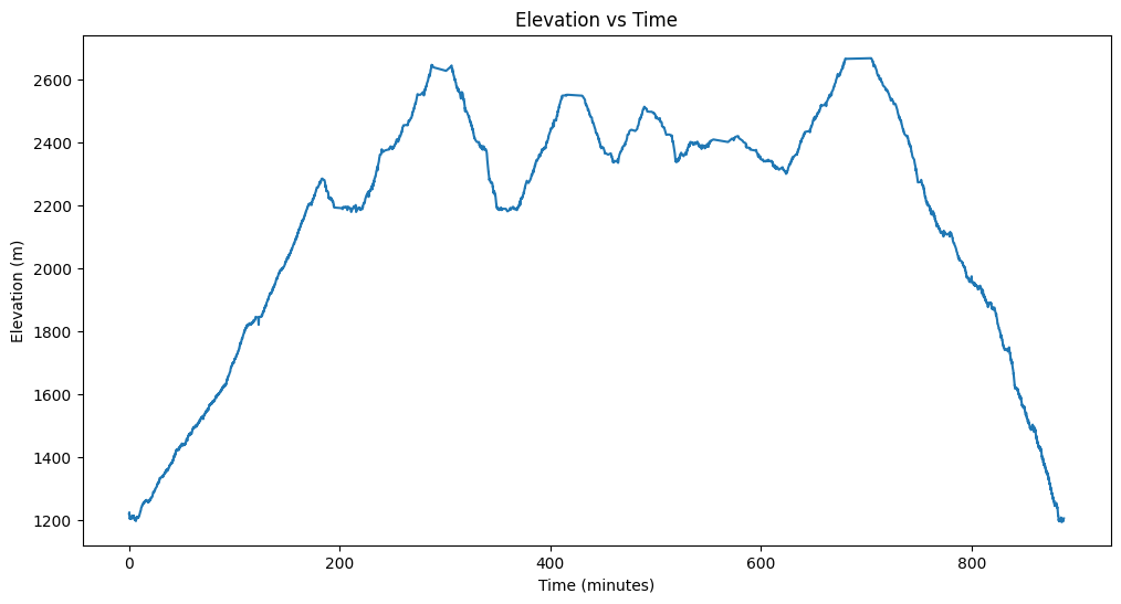
Those flat sections are in order, from left to right: An alpine lake (not really a break, since we had to walk around it), the summit of Star Peak, the alpine lake again, the summit of Courtney peak, and the summit of Oval Peak.

I wrote some code to remove all the sections from this track where I’m stationary (moving at under 0.03 m/s) for 5 minutes or more. Here’s what this “trimmed” track looks like on the same plot:

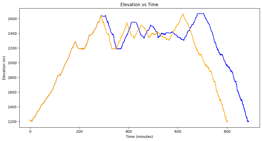
If I check the duration of my new trimmed track, it clocks in at 13h 22m 10s. Dang, still not enough to get an FKT, but maybe I need to start running this script on my Strava activities before I upload them…

Note: The specific thresholds I’m using are total guesses. There is no science here, only art.

How well do the pace functions work on the trimmed tracks?

Hike Tracks

I ran the same error analysis applying on the trimmed tracks. Let’s see what this looks like for Hike Tracks first:

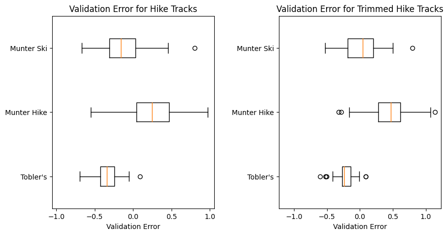
Since this is a little harder to immediately grasp, I’ll also include the raw percentiles:

Error data for hike tracks:

pacefunc	min error	25th percentile error	50th percentile error	75th percentile error	max error	IQR
Tobler’s	-0.6946	-0.42312	-0.341471	-0.241053	0.0923743	0.182067
Munter Hike	-0.551169	0.0422448	0.249435	0.466705	0.972652	0.424461
Munter Ski	-0.6707	-0.310926	-0.157491	0.0320515	0.800865	0.342978

Error data for trimmed hike tracks:

pacefunc	min error	25th percentile error	50th percentile error	75th percentile error	max error	IQR
Tobler’s	-0.600868	-0.269406	-0.236858	-0.140485	0.0923743	0.128921
Munter Hike	-0.323727	0.28344	0.466705	0.617929	1.14304	0.334489
Munter Ski	-0.526672	-0.188644	0.04643	0.203042	0.800865	0.391685

My observations:

For both of our Hiking appropriate functions, errors cluster closer together when evaluating on our trimmed tracks. Munter Ski does slightly worse at clustering, but it’s being used outside of it’s domain.
For toblers, our 50th percentile error got closer to 0, but for Munter, it got further.
Conclusions: Predicting moving time for hikes is “easier” than predicting total time. If you’re going to do it for hiking with one of the standard functions, again, use toblers. It actually works quite well!

Ski Tracks

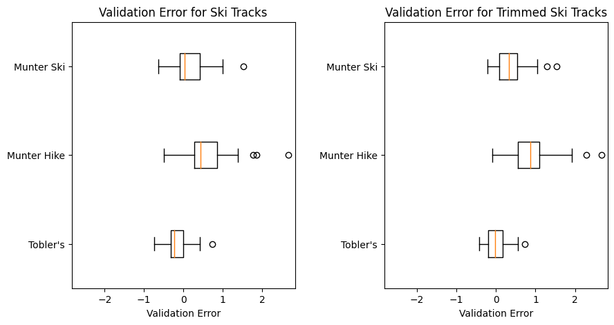
Error data for ski tracks:

pacefunc	min error	25th percentile error	50th percentile error	75th percentile error	max error	IQR
Tobler’s	-0.747568	-0.326341	-0.232423	0.00327991	0.73554	0.32962
Munter Hike	-0.488748	0.285369	0.428108	0.85386	2.66589	0.568492
Munter Ski	-0.639719	-0.0869261	0.0297901	0.422645	1.53325	0.509571

Error data for trimmed ski tracks:

pacefunc	min error	25th percentile error	50th percentile error	75th percentile error	max error	IQR
Tobler’s	-0.424186	-0.196397	-0.0205109	0.175277	0.736631	0.371674
Munter Hike	-0.0999253	0.562524	0.876581	1.10227	2.66774	0.539746
Munter Ski	-0.216255	0.0814588	0.325991	0.536884	1.53483	0.455426

Observations:

Conclusions are far less clear here, trimming the tracks hasn’t really clustered our prediction error any closer, and it took the Munter ski method which previously centered errors around 0 and threw it off.
Tobler’s method is better calibrated on moving time than on total time again.
Recommendations are harder here, since predicting moving time instead of total time doesn’t seem to overall help. Take this as a warning against trusting any of these too much.

Conclusions

Here are some things I’m confident concluding:

It’s easier to accurately estimate travel time for hiking than for backcountry skiing if the only information we have is the profile of the trip. Take this as a warning.
Tobler’s method is better than the Munter method for hike travel time estimation.
It’s easier to predict moving time rather than total time for hiking.

Stay Tuned

I hope to answer at least some of these in a follow-up post.

How much better can we do by fine tuning the parameters? Presumably we can get some improvement
Why is skiing harder to make estimates for? I want to know why exactly our estimates have so much more variation.
Are there other functions we should consider? One obvious idea is a “two-sided” Tobler’s function where the decay rate is different for uphill and downhill. I suspect this may help for skiing.
How weird is my data? Tobler just used data from one of his friends, so his function probably works better for that guy than for me! In particular, I want to know which of the three parameters are “universal” and don’t change much person to person, and which are individually variable. I suspect the base pace is radically different for different people, but for the other two parameters, I have no idea.
Is there some way to normalize for effort? By analyzing data for all my tracks together, I’m ignoring the fact that for some of these I was going full throttle and on others, I was hiking with friends on a lazy Sunday. Maybe I need to try looking at individual tracks. One idea: I could try fitting a pace function on a subset of the chunks for an individual track, then validate on the rest.
Are there good rules of thumb for selecting parameters? It would be really cool if I could give you a function that translates your 5km running time into a RATE parameter that would give you roughly accurate estimates.
How accurate are the Bushwhack parameters? I thankfully have no activities that are 100% Bushwhacking, so I will need to annotate my data to answer this.